The AGILE software with its documentation is available here
This is a schematic view of how the AGILE pipeline works:

Step 1: Creation of the truth catalog containing Galaxies, AGN and stars
- Galaxies: We start from an empirically calibrated galaxy sample with redshifts, stellar masses, star-formation rates, and morphologies generated using EGG (Empirical Galaxy Generator; Schreiber+ 2017) and the most up-to-date measurements of the stellar mass function (COSMOS2020; Weaver+ 2023) up to z ~ 5.5.
- AGN: We then populate galaxies with AGN whose properties are based on empirical recipes:
In detail:
- Galaxies are populated with specific accretion rates lambda_SAR = LX/Mstar according to the p(lambda_SAR = LX / Mstar | Mstar, z, type) by Zou+2024
- X-ray AGN with LX and z are assigned optical type1/type2 following Merloni+2014
- Optical (2500 AA) luminosities are assigned to X-ray AGN based on alpha_OX following the relation by Lusso+2010
- Optical SEDs and broad-band magnitudes are assigned to X-ray AGN according to re-fitted parameters (this work) by QSOGEN (Temple+ 2021)
- AGN E(B-V) is assigned based on empirical distributions from COSMOS (type2) and LSST DDF (type1)
- MBH is assigned according to MBH-Mstar scaling relations based on the continuity model with redshift evolution (Roberts, Shankar, in prep.)
3. Stars: Finally, the Milky Way and Magellanic cloud single and binary stars are added from the publicly available LSST SIM database, which is based on the TRILEGAL code (Girardi+ 2012). Variability is included also for the star catalog.
Step 2: Creation of the instance truth catalog
The second step consists in going from a purely static Universe to a variable one. This is achieved by assigning optical lightcurves to variable sources, i.e. AGN and stars (CCs, LPVs and binary star systems). We do not consider transient phenomena such as supernovae, or tidal disruption events.
Specifically, AGN lightcurves are assigned based on a Damped Random Walk model taking into account physical AGN properties e.g. luminosity and MBH (Suberlak+ 2021)
Step 3: Simulated multi-band LSST images (ugrizy):
The AGN+galaxy+stars truth catalog is then fed into the LSST image simulation pipeline Imsim , which takes into account instrumental effects, sky background, and the LSST cadence, to generate simulated multi-band images in the Rubin-LSST bands, i.e. u, g, r, i, z, y (and possibly also Euclid VIS+NIR bands). For the current release, we have used the LSST baseline 4.0. In Fig. 1 we show the r-band image corresponding to 1 patch (0.05deg2) with overplotted type-1 AGN (orange circles), type-2 AGN (green circles), galaxies (red circles) and stars (violet).
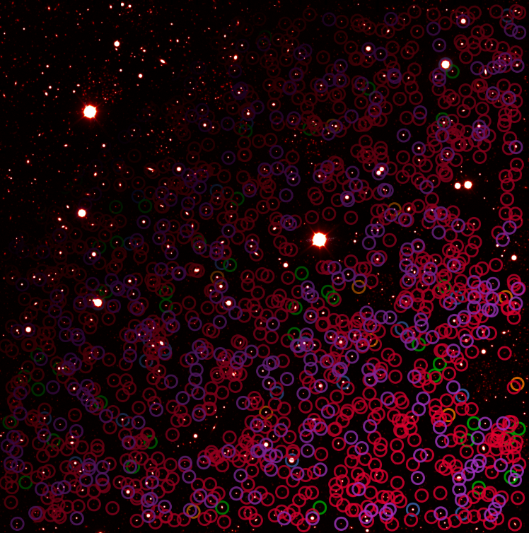
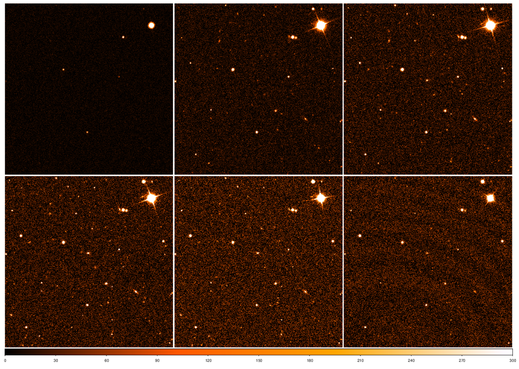
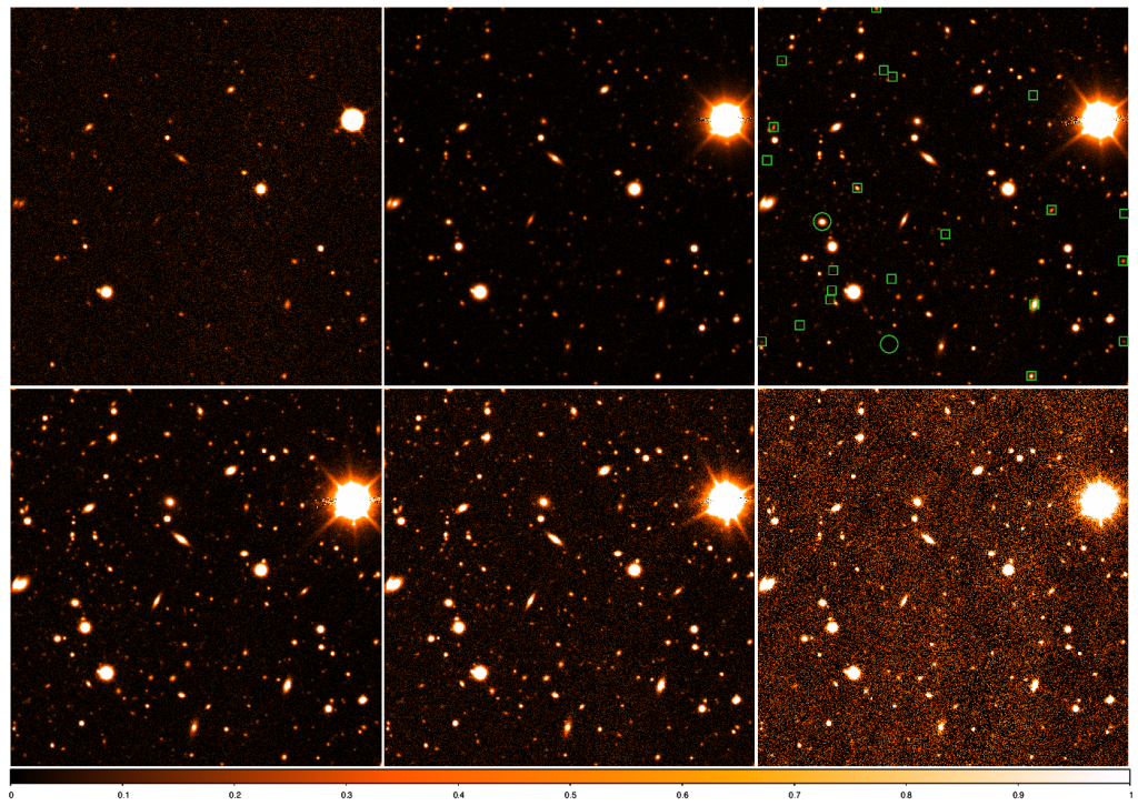
Fig. 2 and 3 show a zoom-in to the individual 30s calexp images and coadded images. The panels correspond to ugrizy (left to right, top to bottom).
Step 4: Building realistic catalog-level simulated data:
On the simulated images we then extract the photometric catalogs using the official LSST photometric tool (https://pipelines.lsst.io/index.html) in order to create a realistic LSST photometric catalog.
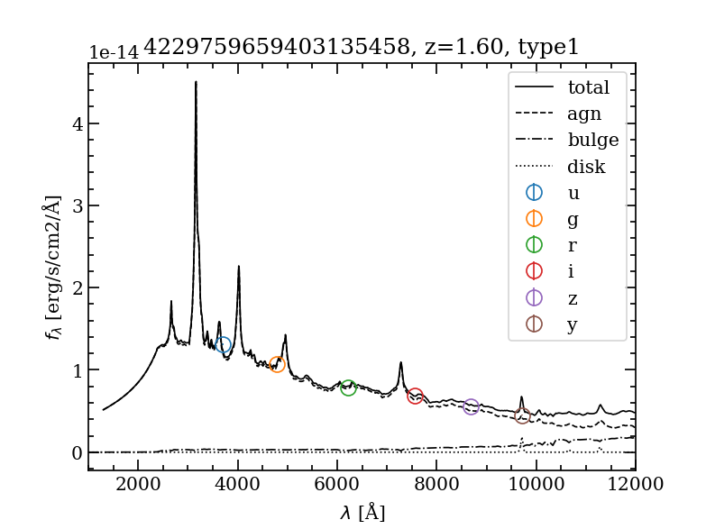
Fig. 4 shows an example of simulated SED (black line) with overplotted the extracted realistic fluxes (circles) while Fig. 5 shows a simulated AGILE type1 AGN lightcurve (solid line) with fluxes (circles) extracted in the imSim simulated images using the LSST Science Pipelines.

The AGILE software with its documentation is available here